PEtab 2.0 tutorial

Overview

In the following, we demonstrate how to set up a parameter estimation problem in PEtab based on a realistic application example. To this end, we consider the model and experimental data by Boehm et al. (2014). The model describes the dynamics of phosphorylation and dimerization of the transcription factors STAT5A and STAT5B. A visualization and the corresponding reactions of the model are provided below, although the details of the model are not relevant for the purpose of this tutorial. For more details, we refer to the original publication.

We will start with the model, and then proceed to link the model to experimental data by defining experimental conditions, observation functions, and measurements. After this, we will define the parameters to be estimated, and finally group all files in a YAML file to define the PEtab problem.

1. The model

PEtab assumes that an SBML file of the model exists. Here, we use the SBML model provided in the original publication, which is also available on Biomodels (https://www.ebi.ac.uk/biomodels/BIOMD0000000591). For illustration purposes we slightly modified the SBML model and shortened some parts of the PEtab files. The full PEtab problem introduced in this tutorial is available online.

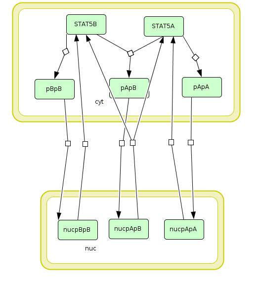
Visualization of the model used as example in this tutorial. The model describes the dynamics of phosphorylation and dimerization of the transcription factors STAT5A and STAT5B.

Reactions included in the example model.

ID	Reaction	Rate law
R1	2 STAT5A → pApA	cyt * BaF3_Epo * STAT5A^2 * k_phos
R2	STAT5A + STAT5B → pApB	cyt * BaF3_Epo * STAT5A * STAT5B * k_phos
R3	2 STAT5B → pBpB	cyt * BaF3_Epo * STAT5B^2 * k_phos
R4	pApA → nucpApA	cyt * k_imp_homo * pApA
R5	pApB → nucpApB	cyt * k_imp_hetero * pApB
R6	pBpB → nucpBpB	cyt * k_imp_homo * pBpB
R7	nucpApA → 2 STAT5A	nuc * k_exp_homo * nucpApA
R8	nucpApB → STAT5A + STAT5B	nuc * k_exp_hetero * nucpApB
R9	nucpBpB → 2 STAT5B	nuc * k_exp_homo * nucpBpB

2. Linking model and measurements

The model by Boehm et al. (2014) was calibrated on measurements on phosphorylation levels of STAT5A and STAT5B as well as relative STAT5A abundance for different timepoints between 0 - 240 minutes after stimulation with erythropoietin (Epo):

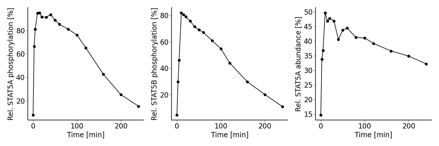
Measurements considered for model calibration in our example.

To define a parameter estimation problem in PEtab, we need to map measurements to the model state. To this end, we need to 1) specify the experimental conditions the measurements were generated from, 2) specify observation functions and error models, and 3) specify the measurements themselves. For this, we need to define observation functions as well as experimental conditions under which a measurement was performed.

2.1 Specifying experimental conditions

All measurements were collected under the same experimental condition, which is a stimulation with Epo. In PEtab, we can define experiments, which are characterized by specific conditions (here: discrete changes) that are applied to the model at certain time points.

In the problem considered here, the relevant the model parameter is Epo_concentration, the initial concentration of Epo, which we want to set to a value of 1.25E-7. Since in this example we include data from only one single experiment, it would not be necessary to specify the condition parameter here, but instead the value could have been also set in the model or in the parameter table. However, the benefit of specifying this change as an experiment is that it allows us to easily add measurements from other experiments performed with different Epo concentrations later on.

We define a single experiment in the PEtab experiment table, a tab-separated values (TSV) file[1]:

Experiment table experiments.tsv.

experimentId	time	conditionId
epo_stimulation	0.0	epo_bolus

This means that in the experiment we call epo_stimulation, at time point 0.0, the condition epo_bolus is applied to the model. The condition itself is defined in the condition table, another TSV file, below.

The condition table specifies the discrete changes to model parameters or model state that are applied when the respective condition is activated. In our example, we only have one condition with a single change that sets the Epo concentration to 1.25E-7:

Conditions table experimental_conditions.tsv.

conditionId	targetId	targetValue
epo_bolus	Epo_concentration	1.25E-7

In more complex scenarios, multiple conditions could be defined here, and targetValue could contain more complex expressions.

2.2 Specifying the observation model

To link the model state to the measurements shown above, we specify observation functions. Additionally, a noise model is be introduced to account for the measurement errors. In PEtab, this is encoded in the observable table:

Observable table observables.tsv.

observableId	observableName	…
pSTAT5A_rel	Rel. STAT5A phosphorylation [%]	…
pSTAT5B_rel	Rel. STAT5B phosphorylation [%]	…
rSTAT5A_rel	Rel. STAT5A abundance [%]	…

Observable table observables.tsv (continued).

…	observableFormula	…
…	100*(2*pApA + pApB) / (2*pApA + pApB + STAT5A)	…
…	100*(2*pBpB + pApB) / (2*pBpB + pApB + STAT5B)	…
…	100*(STAT5A + pApB + 2*pApA) / (2 * pApB + 2* pApA + STAT5A + STAT5B + 2*pBpB)	…

Observable table observables.tsv (continued).

…	noiseFormula	noisePlaceholders	noiseDistribution
…	pSTAT5A_rel_sigma	pSTAT5A_rel_sigma	normal
…	pSTAT5B_rel_sigma	pSTAT5B_rel_sigma	normal
…	rSTAT5A_rel_sigma	rSTAT5A_rel_sigma	normal

• observableId specifies a unique identifier to the observables that can be used to link them to the measurements (see below).

• observableName can be used as a human readable description of the observable.

• observableFormula is a mathematical expression defining how the model output is calculated. The formula can consist of species and parameters defined in the SBML file. In our example, we measure e.g. the relative phosphorylation level of STAT5A (pSTAT5A_rel), which is the sum of all species containing phosphorylated STAT5A over the sum of all species containing any form of STAT5A.

• noiseFormula is used to describe the formula for the measurement noise. Together with noiseDistribution, it defines the noise model. In this example, we assume additive, normally distributed measurement noise. In this scenario, {observableId}_sigma is the standard deviation of the measurement noise. Because we want to estimate the standard deviation from the data, we parameterize it here. Furthermore, we flag these parameters as placeholders in the noisePlaceholders column, which allows us to substitute them with specific values for each measurement in the measurement table (see below).

2.3 Specifying measurements

The experimental data is linked to the experiments via the experimentId and to the observables via the observableId. This is defined in the PEtab measurement file:

Measurement table measurement_data.tsv.

observableId	experimentId	measurement	time	noiseParameters
pSTAT5A_rel	epo_stimulation	7.9	0	sd_pSTAT5A_rel
…	…	…	…	…
pSTAT5A_rel	epo_stimulation	15.4	240	sd_pSTAT5A_rel
pSTAT5B_rel	epo_stimulation	4.6	0	sd_pSTAT5B_rel
…	…	…	…	…
pSTAT5B_rel	epo_stimulation	10.96	240	sd_pSTAT5B_rel
rSTAT5A_rel	epo_stimulation	14.7	0	sd_rSTAT5A_rel
…	…	…	…	…
rSTAT5A_rel	epo_stimulation	32.2	240	sd_rSTAT5A_rel

• observableId references the observableId from the observable file.

• experimentId references the experimentId from the experiment file.

• measurement defines the values that are measured for the respective observable and experiment.

• time is the time point at which the measurement was performed. For brevity, only the first and last time point of the example are shown here (the omitted measurements are indicated by “…” in the example).

• noiseParameters relates to the noiseParameters in the observable table. In our example, the measurement noise is unknown. Therefore we specify parameters here which have to be estimated (see parameters sheet below). If the noise is known, e.g. from multiple replicates, numeric values can be specified in this column.

3. Defining parameters

The model by Boehm et al. (2014) contains nine unknown parameters that need to be estimated from the experimental data. Additionally, it has one known parameter that is fixed to a literature value.

The parameter table for this is given by:

Parameter table parameters.tsv.

parameterId	lowerBound	upperBound	nominalValue	estimate
Epo_degradation_BaF3	1E-5	1E+5		true
k_exp_hetero	1E-5	1E+5		true
k_exp_homo	1E-5	1E+5		true
k_imp_hetero	1E-5	1E+5		true
k_imp_homo	1E-5	1E+5		true
k_phos	1E-5	1E+5		true
ratio			0.693	false
sd_pSTAT5A_rel	1E-5	1E+5		true
sd_pSTAT5B_rel	1E-5	1E+5		true
sd_rSTAT5A_rel	1E-5	1E+5		true

• parameterId references parameters defined in the SBML file or introduced in the condition table or the measurement table. In this example, the first seven parameters are specified in the model, and the last three parameters are the standard deviations for the different observables (sd_{observableId}) that we introduced in the measurement table.

• lowerBound and upperBound define the bounds for the parameters used during estimation. These are usually biologically plausible ranges.

• estimate defines whether the parameter will be estimated (true) or be fixed (false) to the value in the nominalValue column.

• nominalValue are known values used for simulation. The entry can be left empty, if a value is unknown and requires estimation.

5. YAML file

The parameter estimation problem is fully defined by the files created above. However, to facilitate importing the problem into tools supporting PEtab, a YAML file is used to group the files together. This file has the following format (Boehm_JProteomeRes2014.yaml):

format_version: 2.0.0
model_files:
  model:
    location: model_Boehm_JProteomeRes2014.xml
    language: sbml
parameter_files:
  - parameters.tsv
experiment_files:
  - experiments.tsv
condition_files:
  - experimental_conditions.tsv
observable_files:
  - observables.tsv
measurement_files:
  - measurement_data.tsv

The first line specifies the PEtab version this file and the files referenced adhere to. The next block specifies the model file, in this case an SBML file. This is followed by lists of the different PEtab files created above: parameter, experiment, condition, observable, and measurement files. Here, each list contains only one file, but multiple files can be referenced if needed.

7. Further information

This tutorial only demonstrates a subset of PEtab functionality. For full reference, consult the PEtab specification. After finishing the implementation of the PEtab problem, its correctness can be verified using the petablint tool provided by the PEtab Python library (usage). The PEtab problem can then be used as input to the supporting toolboxes to estimate the unknown parameters or calculate parameter uncertainties.

[1]

TSV files can be created using any standard spreadsheet application, or for small files, text editor.

References

• Martin E. Boehm, Lorenz Adlung, Marcel Schilling, Susanne Roth, Ursula Klingmüller, and Wolf D. Lehmann. Journal of Proteome Research 2014 13 (12), 5685-5694. DOI: 10.1021/pr5006923.